Voc segmentation#
There is a dataset that contains images of objects from different classes — the Pascal Visual Object Classes (VOC). This page applies the UNet architecture to that dataset.
import os
import torch
from torch import nn
from torch.utils.data import DataLoader

import torchvision
from torchvision import transforms as T
from torchvision.datasets import VOCSegmentation

import wandb
from PIL import Image
import huggingface_hub
import matplotlib.pyplot as plt


if torch.cuda.is_available():
    DEVICE = torch.device("cuda")
elif torch.backends.mps.is_available():
    DEVICE = torch.device("mps")
else:
    DEVICE = torch.device("cpu")
print("using device", DEVICE)


# Determining where the notebook is run and the corresponding setup. If
# necessary, load all required credentials.
runned_in_free_server = False

if 'KAGGLE_KERNEL_RUN_TYPE' in os.environ:
    print("Runned in Kaggle")
    from kaggle_secrets import UserSecretsClient
    user_secrets = UserSecretsClient()
    wandb_token = user_secrets.get_secret("wandb_token")
    hf_token = user_secrets.get_secret("hf_token")
    runned_in_free_server = True

elif 'COLAB_GPU' in os.environ:
    print("Runned in colab")
    from google.colab import userdata

    wandb_token = userdata.get("wandb_token")
    hf_token = userdata.get("hf_token")
    runned_in_free_server = True

if runned_in_free_server:
    # Downloading extra source files
    !wget https://raw.githubusercontent.com/fedorkobak/knowledge/refs/heads/main/python/torch/examples/unet/unet.py

    wandb.login(key=wandb_token)
    del wandb_token

    huggingface_hub.login(hf_token)
    del hf_token

from unet import (
    Up, Down,
    DoubleConv,
    evaluate,
    run_epoch,
    save_model,
    load_model
)
using device cpu
Dataset#
Consider dataset that we will work with.
data_transforms = torchvision.datasets.vision.StandardTransform(
    T.ToTensor(), T.ToTensor()
)

train_dataset = VOCSegmentation(
    root='./voc_segmentation',
    year='2012',
    image_set='train',
    download=True
)
val_dataset = VOCSegmentation(
    root='./voc_segmentation',
    year='2012',
    image_set='val',
    download=True
)
Using downloaded and verified file: ./voc_segmentation/VOCtrainval_11-May-2012.tar
Extracting ./voc_segmentation/VOCtrainval_11-May-2012.tar to ./voc_segmentation
Using downloaded and verified file: ./voc_segmentation/VOCtrainval_11-May-2012.tar
Extracting ./voc_segmentation/VOCtrainval_11-May-2012.tar to ./voc_segmentation
As is typical in a segmentation task, it contains pictures and arrays of the same size as the labels, where each pixel represents the class of that pixel.
image, target = train_dataset[10]

plt.figure(figsize=(15, 10))

plt.subplot(131)
plt.imshow(image)
plt.title("Image")
plt.axis('off')

plt.subplot(132)
plt.imshow(target)
plt.title("Target")
plt.axis('off')

plt.subplot(133)
plt.imshow(Image.blend(
    im1=image,
    im2=target.convert('RGB'),
    alpha=0.5
))
plt.title("Blend")
plt.axis('off')


plt.show()
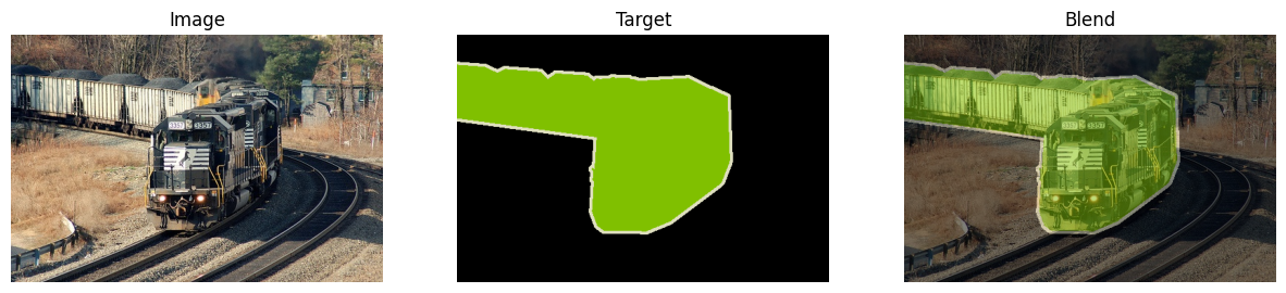
I found the following description of the labels for this task:
1: Aeroplane
2: Bicycle
3: Bird
4: Boat
5: Bottle
6: Bus
7: Car
8: Cat
9: Chair
10: Cow
11: Dining Table
12: Dog
13: Horse
14: Motorbike
15: Person
16: Potted Plant
17: Sheep
18: Sofa
19: Train
20: TV Monitor
But if you check values that are in the target of the arbitrary sample, it will be pictures from 0 to 1, which is not corresponds to the classes description below:
image, target = train_dataset[10]
torch.unique(T.ToTensor()(target))
tensor([0.0000, 0.0745, 1.0000])
The target has to be multiplied by 255 to obtain the labels. The following cell shows the unique numbers and their of the target multiplied by 255 for a purposely selected picture from the training set.
ans = torch.unique(T.ToTensor()(target)*255, return_counts=True)
dict(zip([v.item() for v in ans[0]], [v.item() for v in ans[1]]))
{0.0: 115576, 19.0: 46635, 255.0: 4289}
There are the numbers 0, 19, and 255. The number 19 obviously corresponds to pixels in the train. Based on the counts, it appears that 0 corresponds to the background pixels and 255 corresponds to the border pixels.
According to the information discovered earlier, we are constructing our target values.
transforms = torchvision.datasets.vision.StandardTransform(
    transform=T.Compose([
        T.ToTensor(),
        T.Resize([128, 128], antialias=True),
        T.Lambda(lambda x: x.to(device=DEVICE))
    ]),
    target_transform=T.Compose([
        T.ToTensor(),
        T.Resize([128, 128], antialias=True, interpolation=T.InterpolationMode.NEAREST),
        # After applying `ToTensor`, the target will have one extra dimension
        # for channels, which is ambiguous in this case — that's why we apply
        # `squeeze`.
        T.Lambda(lambda x: x.squeeze()),
        T.Lambda(lambda x: (x*255).long()),
        T.Lambda(lambda x: torch.where(x==255, 21, x)),
        T.Lambda(lambda x: x.to(device=DEVICE))
    ])
)

train_dataset.transforms = transforms
val_dataset.transforms = transforms
The following cell visualizes the data obtained after all transformations.
plt.figure(figsize=(15, 10))

input, target = train_dataset[10]

plt.subplot(131)
plt.imshow(T.ToPILImage()(input))
plt.title("Image")
plt.axis(False)

plt.subplot(132)
plt.imshow(target)
plt.title("Target")
plt.axis(False)

plt.show()
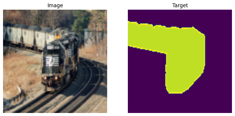
Well, the pictures are now significantly smaller, but they are all the same size.
Model#
class UNet(nn.Module):
    def __init__(self, n_channels, n_classes):
        super(UNet, self).__init__()

        self.n_channels = n_channels
        self.n_classes = n_classes

        self.inc = DoubleConv(n_channels, out_channels=32)
        self.down1 = Down(in_channels=32, out_channels=64)
        self.down2 = Down(in_channels=64, out_channels=128)
        self.down3 = Down(in_channels=128, out_channels=256)

        self.bottleneck = Down(in_channels=256, out_channels=256)

        # Input Up layer is concatenation by channels of the previous layer
        # and corresponding down layer
        self.up1 = Up(in_channels=512, out_channels=128)
        self.up2 = Up(in_channels=256, out_channels=64)
        self.up3 = Up(in_channels=128, out_channels=32)
        self.up4 = Up(in_channels=64, out_channels=32)

        # The last layer applies a convolution that preserves the dimensionality
        # of the feature maps and returns as many channels as the number of
        # predicted classes.
        self.outc = torch.nn.Conv2d(
            in_channels=32,
            out_channels=n_classes,
            kernel_size=1
        )

    def forward(self, x):
        x1 = self.inc(x=x)
        x2 = self.down1(x=x1)
        x3 = self.down2(x=x2)
        x4 = self.down3(x=x3)
        x5 = self.bottleneck(x=x4)
        x = self.up1(x=x5, x_left=x4)
        x = self.up2(x=x, x_left=x3)
        x = self.up3(x=x, x_left=x2)
        x = self.up4(x=x, x_left=x1)
        logits = self.outc(x)
        return logits
Fitting#
The following cell realises fitting procedure that was used ot train the model.
torch.manual_seed(20)

create_model = lambda: UNet(n_channels=3, n_classes=22)
model = create_model()
model.to(DEVICE)

batch_size = 8
learning_rate = 1e-3

wandb.init(
    project="VOCSegmentation",
    config={
        "batch_size": batch_size,
        "learning_rate": learning_rate
    }
)

loss_fun = torch.nn.functional.cross_entropy
optimizer = torch.optim.Adam(params=model.parameters(), lr=learning_rate)

train_loader = DataLoader(train_dataset, batch_size=batch_size)
test_loader = DataLoader(val_dataset, batch_size=batch_size)
best_test_accuracy = 0

try:
    for epoch in range(50):

        run_epoch(
            model=model,
            loader=train_loader,
            loss_fun=loss_fun,
            optimizer=optimizer
        )
        train_accuracy, train_loss = evaluate(
            model=model,
            loader=train_loader,
            loss_fun=loss_fun,
            tqdm_desc="Evaluate train"
        )
        test_accuracy, test_loss = evaluate(
            model=model,
            loader=test_loader,
            loss_fun=loss_fun,
            tqdm_desc="Evaluate test"
        )

        wandb.log(
            {
                "train_loss": train_loss,
                "test_loss": test_loss,
                "train_accuracy": train_accuracy,
                "test_accuracy": test_accuracy
            },
            step=epoch
        )

        if test_accuracy > best_test_accuracy:
            best_test_accuracy = test_accuracy
            best_model = create_model()
            best_model.load_state_dict(model.state_dict())

except KeyboardInterrupt:
    pass
And finally, here’s how you can save the best model to your Hugging Face account.
save_model(model=best_model, name="VOCSegmentatoin.pt")
Evaluating model#
In this section, we will load the best model and evaluate its actual performance.
model = load_model(
    model=UNet(n_channels=3, n_classes=22),
    name="VOCSegmentatoin.pt"
)
model = model.eval()
The following cell represents accuracy of the final model.
test_loader = DataLoader(val_dataset, batch_size=64)
accuracy, _ = evaluate(
    model=model,
    loader=test_loader,
    loss_fun=torch.nn.functional.cross_entropy
)
print(f"Accuracy of the model - {accuracy*100}%")
100%|██████████| 23/23 [01:01<00:00, 2.65s/it]
Accuracy of the model - 65.68055152893066%