Nearest neighbors

Is algorithm that allows to build find closest points

import io
from IPython.display import Image as IPImage

import numpy as np
import pandas as pd

import matplotlib.pyplot as plt

from sklearn.neighbors import NearestNeighbors
from sklearn.datasets import make_blobs

Example

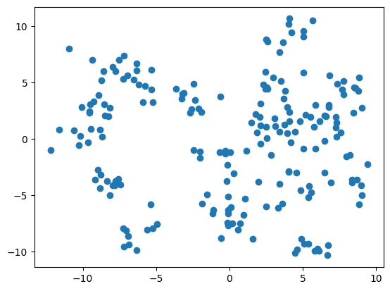
Let’s consider an example - a set of two-dimensional objects that we are going to use among which we need to choose some set of the closest to the given object.

X, _ = make_blobs(
    n_samples=200,
    random_state=10,
    centers=20
)
plt.scatter(X[:,0], X[:,1])
plt.show()

To use sklearn.neighbours.NearestNeighbours we need to define the number of neighbours and apply it to the data under consideration.

nn = NearestNeighbors(n_neighbors=20).fit(X)

kneighbors method

To get predictions, we need to use the kneighbors method on this object. The following example shows oupt for two specified points.

distances, indices = nn.kneighbors([[0,0], [2,2]])
display(pd.concat(
    {
        "distances" : pd.DataFrame(distances.T),
        "idices" : pd.DataFrame(indices.T)
    },
    axis = 1
))

	distances		idices
	0	1	0	1
0	1.091216	0.074815	170	40
1	1.138347	0.302468	118	142
2	1.309527	0.724875	45	10
3	1.336416	0.770803	54	62
4	1.535604	1.045741	71	84
5	1.980926	1.082107	137	122
6	2.103606	1.185385	10	18
7	2.159102	1.392603	151	137
8	2.286014	1.403301	70	51
9	2.294783	1.901535	76	144
10	2.452250	1.964599	62	50
11	2.565371	1.995106	50	149
12	2.629244	2.133964	29	47
13	2.630536	2.136047	46	75
14	2.745844	2.145365	84	11
15	2.853642	2.319772	40	127
16	2.868993	2.435027	142	151
17	3.049752	2.472242	80	128
18	3.080130	2.513303	160	113
19	3.164793	2.517343	166	61

For each object it returns the distances to the neighbours and the indices of the neighbours.

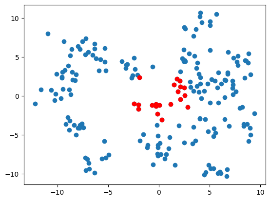
kneighbors_graph method

kneighbors_graph is an alternative way of extracting neighbours. It returns neighbor elements as boolean mapping 1 - means that object corresponds to the set of neighbor objects, 0 doesn’t.

graph = nn.kneighbors_graph([[0,0]]).toarray()[0]
display(graph)
plt.scatter(
    X[:,0], X[:,1]
)
plt.scatter(
    X[graph.astype("bool"),0],
    X[graph.astype("bool"),1],
    color="red"
)
plt.show()

array([0., 0., 0., 0., 0., 0., 0., 0., 0., 0., 1., 0., 0., 0., 0., 0., 0.,
       0., 0., 0., 0., 0., 0., 0., 0., 0., 0., 0., 0., 1., 0., 0., 0., 0.,
       0., 0., 0., 0., 0., 0., 1., 0., 0., 0., 0., 1., 1., 0., 0., 0., 1.,
       0., 0., 0., 1., 0., 0., 0., 0., 0., 0., 0., 1., 0., 0., 0., 0., 0.,
       0., 0., 1., 1., 0., 0., 0., 0., 1., 0., 0., 0., 1., 0., 0., 0., 1.,
       0., 0., 0., 0., 0., 0., 0., 0., 0., 0., 0., 0., 0., 0., 0., 0., 0.,
       0., 0., 0., 0., 0., 0., 0., 0., 0., 0., 0., 0., 0., 0., 0., 0., 1.,
       0., 0., 0., 0., 0., 0., 0., 0., 0., 0., 0., 0., 0., 0., 0., 0., 0.,
       0., 1., 0., 0., 0., 0., 1., 0., 0., 0., 0., 0., 0., 0., 0., 1., 0.,
       0., 0., 0., 0., 0., 0., 0., 1., 0., 0., 0., 0., 0., 1., 0., 0., 0.,
       1., 0., 0., 0., 0., 0., 0., 0., 0., 0., 0., 0., 0., 0., 0., 0., 0.,
       0., 0., 0., 0., 0., 0., 0., 0., 0., 0., 0., 0., 0.])

Visualisation

The next cell represents a set of functions that allows to visualise the results of the nearest neighbours algorithm. It’s often used in notebooks in this section, so it’s stored in a separate module.

%%writefile nearest_neighbors_files/visualisations.py
import io
import PIL
from PIL import Image

import numpy as np
from sklearn.neighbors import NearestNeighbors

import matplotlib.pyplot as plt

def get_picture(
    coordinates : list[float],
    nn : NearestNeighbors,
    X : np.array,
    title : str
) -> PIL.PngImagePlugin.PngImageFile:
    '''
    Get picture that show neighbours
    for given coordinates.

    Parameters
    ----------
    coordinates : list[float]
        сoordinates for which you need 
        to find neighbours;
    nn : sklearn.neighbors.NearestNeighbors
        algorithm under consideration;
    X : np.array of shape (n_samples, 2)
        this is two dimentional objects
        that will be represented at the
        scatter plot;
    title : str
        title that will be used for plot.

    Returns
    -------
    out : PIL.PngImagePlugin.PngImageFile
        picture with scatters.
    '''
    
    # getting neighrours
    distances, indices = nn.kneighbors([coordinates])

    # plotting scatter
    fig, ax = plt.subplots()
    ax.scatter(
        coordinates[0],
        coordinates[1],
        color="Green",
        s=100
    )
    ax.scatter(X[:,0], X[:,1])
    ax.scatter(X[indices, 0], X[indices, 1], color="red")
    plt.title(title)
    
    # saving to buffer
    buf = io.BytesIO()
    plt.savefig(buf, format='png')
    buf.seek(0)
    plt.close(fig)

    return Image.open(buf)

def get_gif(
    coordinates : list[list[float]], 
    nn : NearestNeighbors, 
    X : np.array,
    pictures_args : dict = {}
)->io.BytesIO:
    '''
    Get buffer containing gif
    file with animation where point 
    for which neighbours, moving
    according to given array.

    Parameters
    ----------
    coordinates : list[list[float]]
        array of coordinate combinations 
        along which the point will move 
        and for which we need to find neighbours;
    nn : sklearn.neighbors.NearestNeighbors
        algorithm under consideration;
    X : np.array of shape (n_samples, 2)
        this is two dimentional objects
        that will be represented at the
        scatter plot;
    pictures_args : dict
        this funciton is wrapper under get_picture
        so you can specify arguemnst to it.
    '''
    # generate frames on which the 
    # coordinate to which neighbours 
    # are searched moves in a circle.
    frames = [
        get_picture(
            coordinates=cord,
            nn=nn,
            X=X,
            **pictures_args
        )
        for cord in coordinates
    ]

    # creating buffer with gif file
    # and displaying it
    gif_buf = io.BytesIO()
    frames[0].save(
        gif_buf, 
        format='GIF', 
        save_all=True, 
        append_images=frames[1:], 
        duration=100, 
        loop=0
    )
    gif_buf.seek(0)
    return gif_buf

def get_circle_gif(
    nn : NearestNeighbors,
    X : np.array,
    radius : float = 5, 
    frames : int = 100,
    center : list = [0,0],
    pictures_args : dict = {}
)->io.BytesIO:
    '''
    Visualises the nearest neighbours to a 
    point that walks in a circle.

    Parameters
    ----------
    nn : sklearn.neighbors.NearestNeighbors
        algorithm under consideration;
    X : np.array of shape (n_samples, 2)
        this is two dimentional objects
        that will be represented at the
        scatter plot;
    radius : float, default=5
        radius of the circle;
    frames : int, deafult=5
        number of frames that will
        be used to build the gif;
    center : list[float] of len 2, default=[0,0]
        center of the circle;
    pictures_args : dict
        this funciton is wrapper under get_picture
        so you can specify arguemnst to it.
    '''
    return get_gif(
        coordinates=[
            [
                center[0] + np.cos(angle)*radius, 
                center[1] + np.sin(angle)*radius
            ]
            for angle in np.linspace(0, 2*np.pi, frames)
        ],
        nn=nn, X=X,
        pictures_args=pictures_args,
    )

Overwriting nearest_neighbors_files/visualisations.py

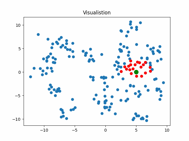
Here is an animation showing the result of the algorithm for different positions of the considered point (green point). The closest neighbours at any time are shown as red dots.

import nearest_neighbors_files.visualisations as visualisations
gif_buf = visualisations.get_circle_gif(
    nn, X,
    pictures_args=dict(
        title="Visualistion"
    )
)
IPImage(data=gif_buf.getvalue())