CNN classification

The process of building a convolutional neural network for image classification is described here.

import numpy as np

import torch
from torch import nn
from torch.utils.data import DataLoader

import torchvision.transforms as T
from torchvision.datasets import CIFAR10

import pickle
from tqdm import tqdm
import matplotlib.pyplot as plt
from IPython.display import clear_output
from tempfile import TemporaryDirectory

from pathlib import Path
files_path = Path("cnn_classification_files")
cifar_path = files_path/"cifar10"

from huggingface_hub import HfApi
from huggingface_hub import hf_hub_download
hf_api = HfApi()

Data

For this notebook, CIFAR10 is used. So it’s loaded in the following cell.

train_dataset = CIFAR10(
    str(cifar_path), 
    train=True, 
    transform=T.ToTensor(),
    download = True
)
valid_dataset = CIFAR10(
    str(cifar_path), 
    train=False,
    transform=T.ToTensor(),
    download=True
)

Files already downloaded and verified
Files already downloaded and verified

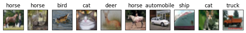
So here is some pictures each belongs to some class. Below is visualisation that contains random picutres from sample with it classes in title.

np.random.seed(15)
indx = np.random.choice(np.arange(len(train_dataset)), 10)
t = [train_dataset[i] for i in indx]

cifar10_classes = {
    0: 'airplane',
    1: 'automobile',
    2: 'bird',
    3: 'cat',
    4: 'deer',
    5: 'dog',
    6: 'frog',
    7: 'horse',
    8: 'ship',
    9: 'truck'
}

plt.figure(figsize = (10, 5))
for i in range(len(indx)):

    plt.subplot(1, len(indx), i + 1)
    plt.title(cifar10_classes[t[i][1]])
    plt.imshow(T.ToPILImage()(t[i][0]))
    plt.xticks([]);plt.yticks([])

There are some tricks at the data level:

• Both training and validation data need to be better normalised;

• For the training data, we added some augmentations that usually make the model more robust.

means = (train_dataset.data / 255).mean(axis=(0, 1, 2))
stds = (train_dataset.data / 255).std(axis=(0, 1, 2))

train_transforms = T.Compose(
    [
        T.AutoAugment(T.AutoAugmentPolicy.CIFAR10),
        T.ToTensor(),
        T.Normalize(mean=means, std=stds)
    ]
)

test_transforms = T.Compose(
    [
        T.ToTensor(),
        T.Normalize(mean=means, std=stds)
    ]
)

train_dataset = CIFAR10(
    str(cifar_path), 
    train=True, 
    transform=train_transforms,
    download = True
)
valid_dataset = CIFAR10(
    str(cifar_path), 
    train=False,
    transform=test_transforms,
    download=True
)

Files already downloaded and verified
Files already downloaded and verified

Architecture

I borrowed the architecture from this notebook.

def conv_block(in_channels, out_channels, pool=False):
    layers = [
        nn.Conv2d(in_channels, out_channels, kernel_size=3, padding=1), 
        nn.BatchNorm2d(out_channels), 
        nn.ReLU(inplace=True)
    ]
    if pool: layers.append(nn.MaxPool2d(2))
    return nn.Sequential(*layers)

class Model(nn.Module):
    def __init__(self, in_channels, num_classes):
        super().__init__()
        
        self.conv1 = conv_block(in_channels, 64)
        self.conv2 = conv_block(64, 128, pool=True)
        self.res1 = nn.Sequential(
            conv_block(128, 128), 
            conv_block(128, 128)
        )
        
        self.conv3 = conv_block(128, 256, pool=True)
        self.conv4 = conv_block(256, 512, pool=True)
        self.res2 = nn.Sequential(
            conv_block(512, 512), 
            conv_block(512, 512)
        )
        
        self.classifier = nn.Sequential(
            nn.MaxPool2d(4), 
            nn.Flatten(), 
            nn.Linear(512, num_classes)
        )
        
    def forward(self, xb):
        out = self.conv1(xb)
        out = self.conv2(out)
        out = self.res1(out) + out
        out = self.conv3(out)
        out = self.conv4(out)
        out = self.res2(out) + out
        out = self.classifier(out)
        return out

Fitting

Here is everything we needed to make the model fit. Everything is quite simple except learning the scheduler. It’s a tool that allows to reduce the steps of the optimiser to get better optimisation results.

device = torch.device('cuda:0' if torch.cuda.is_available() else 'cpu')
model = Model(3, 10).to(device)
optimizer = torch.optim.Adam(model.parameters(), lr=1e-3)
scheduler = torch.optim.lr_scheduler.StepLR(optimizer, step_size=15, gamma = 0.5)
loss_fn = nn.CrossEntropyLoss()

train_loader = DataLoader(
    train_dataset, 
    batch_size=256, 
    shuffle=True, 
    num_workers=4, 
    pin_memory=True
)
valid_loader = DataLoader(
    valid_dataset, 
    batch_size=256, 
    shuffle=False, 
    num_workers=4, 
    pin_memory=True
)

def train(model) -> tuple[float, float]:
    model.train()

    train_loss = 0
    total = 0
    correct = 0

    for x, y in tqdm(train_loader, desc='Train'):
        x, y = x.to(device), y.to(device)

        optimizer.zero_grad()

        output = model(x)

        loss = loss_fn(output, y)

        train_loss += loss.item()

        loss.backward()

        optimizer.step()
        
        _, y_pred = torch.max(output, 1)
        total += y.size(0)
        correct += (y_pred == y).sum().item()

    train_loss /= len(train_loader)
    accuracy = correct / total

    return train_loss, accuracy


@torch.inference_mode()
def evaluate(model, loader) -> tuple[float, float]:
    model.eval()

    total_loss = 0
    total = 0
    correct = 0

    for x, y in tqdm(loader, desc='Evaluation'):
        x, y = x.to(device), y.to(device)

        output = model(x)

        loss = loss_fn(output, y)

        total_loss += loss.item()

        _, y_pred = torch.max(output, 1)
        total += y.size(0)
        correct += (y_pred == y).sum().item()

    total_loss /= len(loader)
    accuracy = correct / total

    return total_loss, accuracy

def plot_stats(
    train_loss: list[float],
    valid_loss: list[float],
    train_accuracy: list[float],
    valid_accuracy: list[float],
    title: str
):
    plt.figure(figsize=(15, 18))

    plt.subplot(211)
    plt.title(title + ' loss')
    plt.plot(train_loss, label='Train loss')
    plt.plot(valid_loss, label='Valid loss')
    plt.legend()
    plt.grid()


    plt.subplot(212)
    plt.title(title + ' accuracy')
    plt.plot(train_accuracy, label='Train accuracy')
    plt.plot(valid_accuracy, label='Valid accuracy')
    plt.legend()
    plt.grid()

This model fitting requires a noticeable amount of computation, but we have calculated everything and saved the results, the next cell just shows the code used for training.

history = {
    "train_loss" : [],
    "valid_loss" : [],
    "train_accuracy" : [],
    "valid_accuracy" : []
}

for epoch in range(50):
    train_loss, train_accuracy = train(model)
    valid_loss, valid_accuracy = evaluate(model, valid_loader)

    history["train_loss"].append(train_loss)
    history["valid_loss"].append(valid_loss)

    history["train_accuracy"].append(train_accuracy)
    history["valid_accuracy"].append(valid_accuracy)

    clear_output()

    plot_stats(
        history["train_loss"], history["valid_loss"],
        history["train_accuracy"], history["valid_accuracy"],
        "Learning curves"
    )
    plt.show()

    scheduler.step()

Saving results: the model is uploaded to the Hugging Face Hub, while the fitting progress is saved to disk.

with TemporaryDirectory() as tmpdir:
    torch.save(model.state_dict(), Path(tmpdir)/"cnn_classification.pt")
    hf_api.upload_folder(
        repo_id="fedorkobak/knowledge", 
        folder_path=tmpdir
    )

pickle.dump(history, open("cnn_classification_files/fit_history.pck", "wb"))

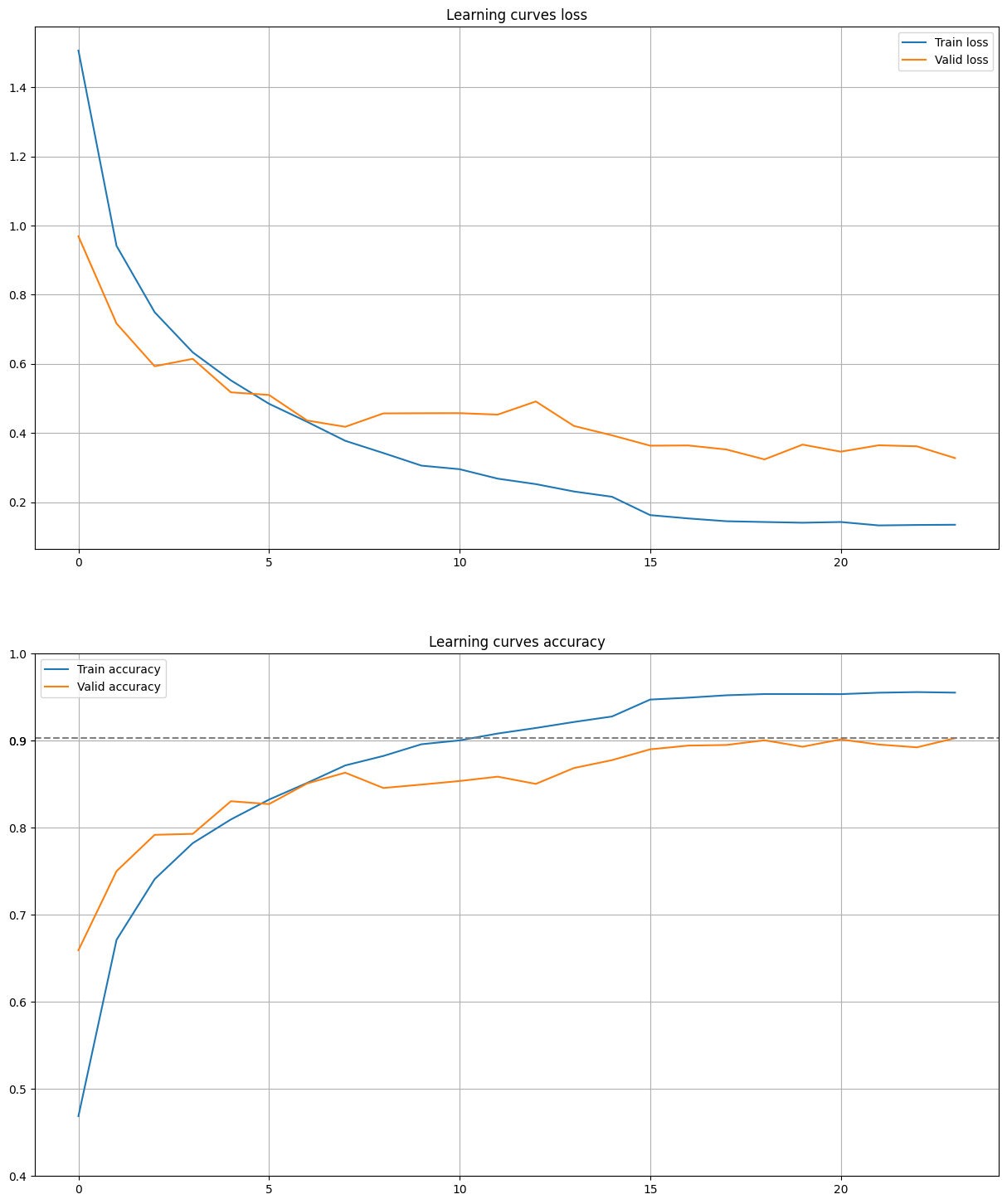
Here is plotted learning curves for model. As you can see the final accuracy is 90%.

history = pickle.load(open("cnn_classification_files/fit_history.pck", "rb"))

plot_stats(
    history["train_loss"], history["valid_loss"],
    history["train_accuracy"], history["valid_accuracy"],
    "Learning curves"
)

final_accuracy = history["valid_accuracy"][-1]
plt.axhline(final_accuracy, color="gray", linestyle="--")

plt.yticks(list(plt.yticks()[0]) + [round(final_accuracy, 2)])
plt.show()

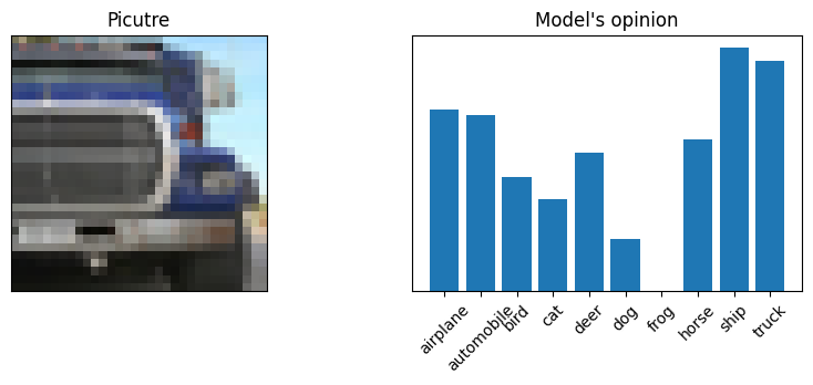
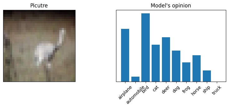
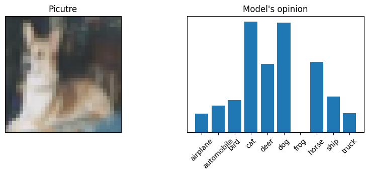
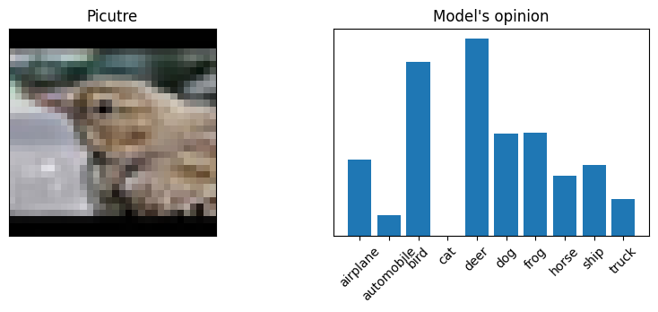
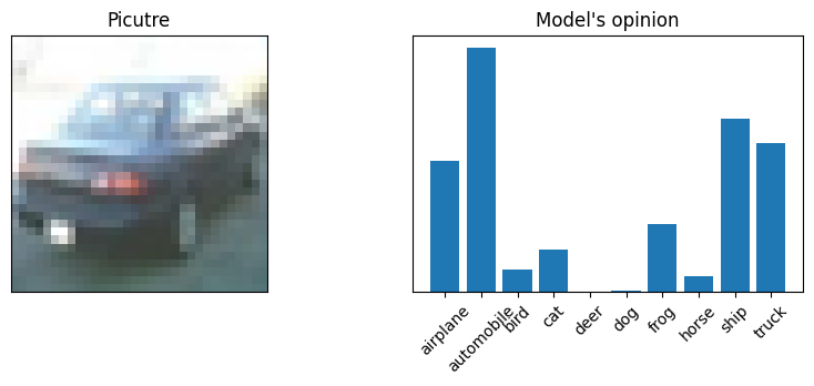
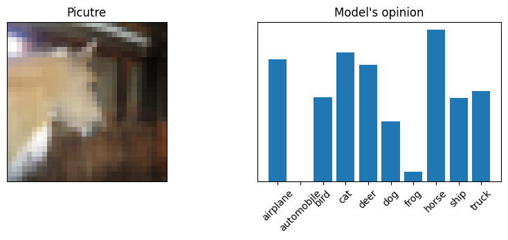
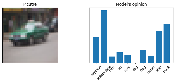
Playing with model

Let’s check models accruraby but not with strickt metric, but with our eyes. Sometimes it’s ever for numan hard to understand what exactly displayed on 32x32 piture. So let’s see what model thinks but not strict classes, but the ratio of model certainties in different classes.

Here is fitted model so you can just download it and do what ever you want.

model = Model(3, 10)

cached_model = hf_hub_download(
    repo_id="fedorkobak/knowledge", 
    filename='cnn_classification.pt'
)
model.load_state_dict(torch.load(cached_model))

model = model.eval()

no_transform_valid = CIFAR10(
    str(cifar_path), 
    train=False,
    download=True
)

indx = np.random.choice(np.arange(len(no_transform_valid)), 10)
predicts = model(
    torch.stack(
        [train_transforms(no_transform_valid[i][0]) for i in indx]
    )
)

predicts

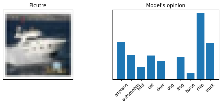
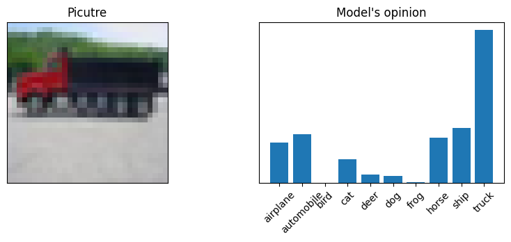
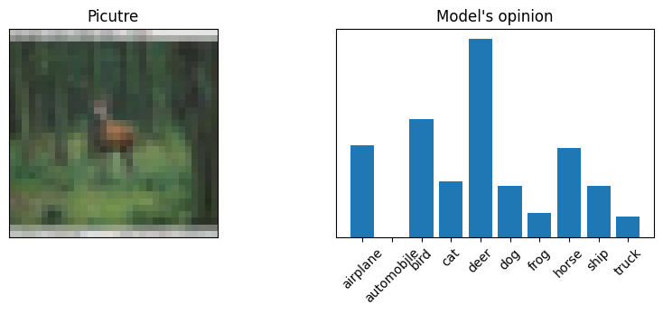
for n, i in enumerate(indx):
    plt.figure(figsize = (10, 3))
    
    plt.subplot(121)
    plt.title("Picutre")
    plt.imshow(no_transform_valid[i][0])
    plt.xticks([]); plt.yticks([])
    
    plt.subplot(122)
    plt.title("Model's opinion")
    plt.bar(
        cifar10_classes.values(), 
        (predicts[n] + predicts[n].min().abs()).detach().numpy()
    )
    plt.xticks(rotation = 45);plt.yticks([])
    plt.show()

Files already downloaded and verified