Metric

sklearn.neighbours.NearestNeighbours has a really important argument - metric, it specifies the formula that will be used to compare objects.

You can pass:

• One of the predefined strings, checkout their list;

• Or callable that takes two arrays representing 1D vectors as inputs and must return one value indicating the distance between those vectors, there are many such options in scipy distance computations.

import os
import sys

from IPython.display import Image as IPImage

import numpy as np
import pandas as pd

import matplotlib.pyplot as plt

from sklearn.neighbors import NearestNeighbors
from sklearn.datasets import make_blobs

from scipy.spatial.distance import correlation

from pathlib import Path
nn_files = Path(os.getcwd()).parent/"nearest_neighbors_files"

if str(nn_files) not in sys.path:
    sys.path.append(str(nn_files))

from visualisations import get_circle_gif

Example

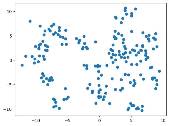
We will use two-dimensional objects to be able to visualise. The following cell generates and visualises the set of objects we are going to use.

X, _ = make_blobs(
    n_samples=200,
    random_state=10,
    centers=20
)
plt.scatter(X[:,0], X[:,1])
plt.show()

Estimators

Now let’s build two estimators - almost the same, just using a different metric. First is using default parameter which is lead to euclidian distance. Second is using scipy.spatial.distance.correlation.

default_metric = NearestNeighbors(n_neighbors=20).fit(X)
correlation_metric = NearestNeighbors(
    n_neighbors=20, 
    metric=correlation
).fit(X)

Now let’s consider what objects will be considered as nearest when using different metrics for an object that walks in a circle.

gif_buf = get_circle_gif(
    default_metric, X,
    pictures_args=dict(
        title="Euclidian"
    )
)
display(IPImage(data=gif_buf.getvalue()))
gif_buf = get_circle_gif(
    correlation_metric, X,
    pictures_args=dict(
        title="Correlation"
    )
)
display(IPImage(data=gif_buf.getvalue()))