Central limit theorem

Formulation

Let’s take \(N\) independent values \(x_i\) belonging to the same distribution with mathematical expectation \(\mu\) and standard deviation \(\sigma\).

Let’s denote their sum:

\[S_N = \sum_{i=1}^n x_i\]

Central limit theorem says that \(S_N \sim N(\mu N; \sigma^2 N)\) (\(S_N\) belongs to normal distibution with parameters \(\mu N, \sigma^2 N\)).

Numerical proof

Let’s create samples of means of samples from different distributions and explore their characteristics.

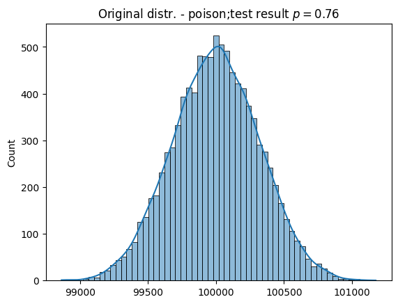
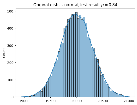
We will plot the histogram of the sample of sums and perform the Cramér-von Mises test to understand if \(S_N\) belongs to the normal distribution.

The \(H_0\) of the Cramér-von Mises test in our case is that \(S_N\) is normally distributed, so if \(p>0.05\) we cannot reject this hypothesis.

import numpy as np

import scipy
from scipy.stats import shapiro, anderson
from scipy.stats import cramervonmises

import seaborn as sns
import matplotlib.pyplot as plt

def explore_is_normal(
    mu : float, sigma : float, 
    sample : np.array, orig_distr_name: str
    ):
    """
    Function that returns whether the given sample
    belongs to the normal distribution. It plots the
    histogram of the distribution and prints the result of the
    of the Cramér-von Mises test in the title.
    Parameters
    ----------
    mu (float) : mathematical expectation of original random value;
    sigma (float) : standart deviation of original random value;
    sample (numpy.array) : sample of sums of original samples;
    orig_distr_name (str) : name of original distribution
        will be pritned on the title of the figure.

    Returns
    ---------
    Plotted histogram of exploring sample.
    """
    s_len = len(sample)
    test_p = cramervonmises(
        sample,
        cdf=scipy.stats.norm(
            mu*s_len,sigma*(s_len**(1/2))
        ).cdf
    ).pvalue
    
    sns.histplot(sample, kde=True)
    plt.title(
        f"Original distr. - {orig_distr_name};" 
        f" Test result $p={str(round(test_p,2))}$"
    )

Normal distribution

This shows that the sum of the random values sampled from the normal distribution belongs to the normal distribution.

sample = np.random.normal(
    2, 3, (10000, 10000)
).sum(axis = 1)
explore(2, 3, sample, "normal")

Poisson distribution

For this research, it is important that this distribution parameters are \(\mu=\lambda\) and \(\sigma=\sqrt{\lambda}\).

_lambda = 10
sample = np.random.poisson(
    _lambda, (10000, 10000)
).sum(axis = 1)
explore(_lambda, _lambda**(1/2), sample, "poison")